Hierarchical Bayesian Model for Binary Responses
Kristian Brock
2020-10-15
Source:vignettes/A500-HierarchicalBayesianResponse.Rmd
A500-HierarchicalBayesianResponse.RmdHierarchical Bayesian model for binary responses
Thall et al. (2003) described a method for analysing treatment effects of a common intervention in several sub-types of a single disease. The treatment effects are assumed to be different but exchangeable and correlated. Observing good efficacy in one cohort, for example, increases one’s expectations of efficacy in other cohorts.
They demonstrate the hierarchical model in a trial with binary response outcomes and in another with time-to-event outcomes. This vignette describes the sarcoma example with binary response outcomes. The authors provide WinBUGS code in the appendix of their paper (Thall et al. 2003). We port their model to Stan and illustrate usage with the example given in their paper.
Implementation in trialr
Statistically, the authors assume that in a trial of \(k\) disease subtypes, the treatment effects are drawn from the same common normal distribution
\(\rho_1, ..., \rho_k \sim N(\mu, \sigma^2)\)
As is the convention in BUGS, the authors define normal distributions by a precision parameter \(\tau\) as opposed to the standard deviation parameter \(\sigma\) used here. We have re-specified the model to comply with the Stan convention of using standard deviation. The authors use a normal hyperprior on \(\mu\), and a gamma hyperprior on \(\tau\), equivalent to an inverse gamma hyperprior on \(\sigma^2\).
We observe \(x_i\) responses in \(n_i\) patients in disease sub-type \(i\). The rate of response in subtype \(i\) is modelled as \(p_i = \text{logit}^{-1}(\rho_i)\). Each \(x_i\) is assumed to be binomially distributed with success parameter \(p_i\). In Stan, that relationship is described as x ~ binomial_logit(n, rho);
The treatment is judged to be worthy of further investigation in cohort \(i\) if
\(\text{Pr}\left\{ p_i > \theta | \mathcal{D} \right\} > q\)
where \(\theta\) is the minimum required response rate, and \(q\) is the required certainty to approve. In their provided example, Thall et al. (2003) use \(\theta = 0.3\).
Example
library(trialr)
We reproduce Thall etl al.’s example. We have outcomes in 10 disease subgroups. The number of responses is stored in group_responses and the number of patients in group_sizes. There have been 3 / 7 responses in subgroup 4, for example, but 0 / 2 responses in subgroup 2, and zero patients treated at all in subgroups 1, 6 and 10.
fit <- stan_hierarchical_response_thall(
  group_responses = c(0, 0, 1, 3, 5, 0, 1, 2, 0, 0),
  group_sizes = c(0, 2 ,1, 7, 5, 0, 2, 3, 1, 0),
  mu_mean = -1.3863,
  mu_sd = sqrt(1 / 0.1),
  tau_alpha = 2,
  tau_beta = 20)
fit## Inference for Stan model: ThallHierarchicalBinary.
## 4 chains, each with iter=2000; warmup=1000; thin=1;
## post-warmup draws per chain=1000, total post-warmup draws=4000.
##
## mean se_mean sd 2.5% 25% 50% 75% 97.5% n_eff
## mu -0.04 0.03 1.41 -2.90 -0.97 -0.01 0.90 2.65 2310
## sigma2 12.39 0.36 11.55 3.20 6.25 9.29 14.73 39.23 1034
## rho[1] -0.06 0.06 3.73 -7.60 -2.27 0.04 2.31 6.99 3622
## rho[2] -2.96 0.07 2.61 -9.44 -4.14 -2.51 -1.23 0.69 1468
## rho[3] 2.36 0.06 2.68 -1.74 0.56 1.98 3.74 8.83 2364
## rho[4] -0.31 0.01 0.77 -1.84 -0.82 -0.29 0.21 1.17 3253
## rho[5] 3.66 0.06 2.26 0.65 2.11 3.19 4.69 9.39 1684
## rho[6] -0.09 0.07 3.63 -7.43 -2.29 -0.09 2.12 7.24 2852
## rho[7] -0.04 0.02 1.51 -3.05 -0.98 -0.01 0.89 2.91 3885
## rho[8] 0.75 0.02 1.28 -1.55 -0.09 0.69 1.50 3.63 3475
## rho[9] -2.41 0.07 2.89 -9.19 -3.80 -1.95 -0.50 1.90 1783
## rho[10] -0.07 0.07 3.76 -7.91 -2.25 -0.03 2.21 7.42 3132
## sigma 3.31 0.04 1.20 1.79 2.50 3.05 3.84 6.26 955
## prob_response[1] 0.50 0.01 0.38 0.00 0.09 0.51 0.91 1.00 3693
## prob_response[2] 0.15 0.00 0.19 0.00 0.02 0.07 0.23 0.66 3775
## prob_response[3] 0.77 0.00 0.25 0.15 0.64 0.88 0.98 1.00 3966
## prob_response[4] 0.43 0.00 0.17 0.14 0.31 0.43 0.55 0.76 3239
## prob_response[5] 0.92 0.00 0.10 0.66 0.89 0.96 0.99 1.00 4917
## prob_response[6] 0.49 0.01 0.38 0.00 0.09 0.48 0.89 1.00 2881
## prob_response[7] 0.49 0.00 0.26 0.05 0.27 0.50 0.71 0.95 4139
## prob_response[8] 0.64 0.00 0.22 0.18 0.48 0.66 0.82 0.97 3778
## prob_response[9] 0.23 0.00 0.25 0.00 0.02 0.12 0.38 0.87 3384
## prob_response[10] 0.50 0.01 0.38 0.00 0.10 0.49 0.90 1.00 2820
## lp__ -34.17 0.13 3.60 -42.60 -36.19 -33.71 -31.52 -28.63 761
## Rhat
## mu 1
## sigma2 1
## rho[1] 1
## rho[2] 1
## rho[3] 1
## rho[4] 1
## rho[5] 1
## rho[6] 1
## rho[7] 1
## rho[8] 1
## rho[9] 1
## rho[10] 1
## sigma 1
## prob_response[1] 1
## prob_response[2] 1
## prob_response[3] 1
## prob_response[4] 1
## prob_response[5] 1
## prob_response[6] 1
## prob_response[7] 1
## prob_response[8] 1
## prob_response[9] 1
## prob_response[10] 1
## lp__ 1
##
## Samples were drawn using NUTS(diag_e) at Thu Oct 15 09:55:32 2020.
## For each parameter, n_eff is a crude measure of effective sample size,
## and Rhat is the potential scale reduction factor on split chains (at
## convergence, Rhat=1).The probability of response in each subgroup is calculated under prob_response. We can use the generic summary function from rstan to get a nice summary:
knitr::kable(rstan::summary(fit, par = 'prob_response')$summary, digits = 3)
| mean | se_mean | sd | 2.5% | 25% | 50% | 75% | 97.5% | n_eff | Rhat | |
|---|---|---|---|---|---|---|---|---|---|---|
| prob_response[1] | 0.502 | 0.006 | 0.381 | 0.001 | 0.094 | 0.511 | 0.910 | 0.999 | 3692.956 | 0.999 |
| prob_response[2] | 0.154 | 0.003 | 0.186 | 0.000 | 0.016 | 0.075 | 0.226 | 0.665 | 3774.893 | 1.000 |
| prob_response[3] | 0.774 | 0.004 | 0.251 | 0.149 | 0.636 | 0.878 | 0.977 | 1.000 | 3965.829 | 1.000 |
| prob_response[4] | 0.433 | 0.003 | 0.168 | 0.137 | 0.306 | 0.428 | 0.552 | 0.762 | 3239.325 | 1.000 |
| prob_response[5] | 0.923 | 0.001 | 0.098 | 0.656 | 0.892 | 0.960 | 0.991 | 1.000 | 4917.029 | 0.999 |
| prob_response[6] | 0.491 | 0.007 | 0.378 | 0.001 | 0.092 | 0.478 | 0.893 | 0.999 | 2881.032 | 1.001 |
| prob_response[7] | 0.494 | 0.004 | 0.265 | 0.045 | 0.272 | 0.498 | 0.710 | 0.949 | 4139.442 | 1.000 |
| prob_response[8] | 0.637 | 0.004 | 0.222 | 0.176 | 0.476 | 0.665 | 0.818 | 0.974 | 3777.952 | 1.000 |
| prob_response[9] | 0.230 | 0.004 | 0.254 | 0.000 | 0.022 | 0.124 | 0.378 | 0.870 | 3384.328 | 1.001 |
| prob_response[10] | 0.495 | 0.007 | 0.379 | 0.000 | 0.095 | 0.493 | 0.901 | 0.999 | 2820.469 | 1.000 |
Let us say that we are willing to approve the treatment for further study in a subgroup if we have at least \(q = 70\)% certainty that the probability of efficacy exceeds the target response rate of 30%.
colMeans(as.data.frame(fit, pars = 'prob_response') > 0.3)
##  prob_response[1]  prob_response[2]  prob_response[3]  prob_response[4]
##           0.60325           0.18100           0.92200           0.76075
##  prob_response[5]  prob_response[6]  prob_response[7]  prob_response[8]
##           1.00000           0.59450           0.71625           0.91175
##  prob_response[9] prob_response[10]
##           0.31000           0.59975
On that basis, at this interim stage, we would be eager to approve the treatment in subgroups 3, 5 and 8. Subgroups 4 and 7 are close to the boundary.
Some distribution plots of the probabilities of efficacy in some subgroups may be informative.
library(ggplot2)
library(rstan)
library(dplyr)

plot(fit, pars = 'prob_response') +
  geom_vline(xintercept = 0.3, col = 'orange', linetype = 'dashed') +
  labs(title = 'Partially-pooled analysis of response rate in 10 sarcoma subtypes')
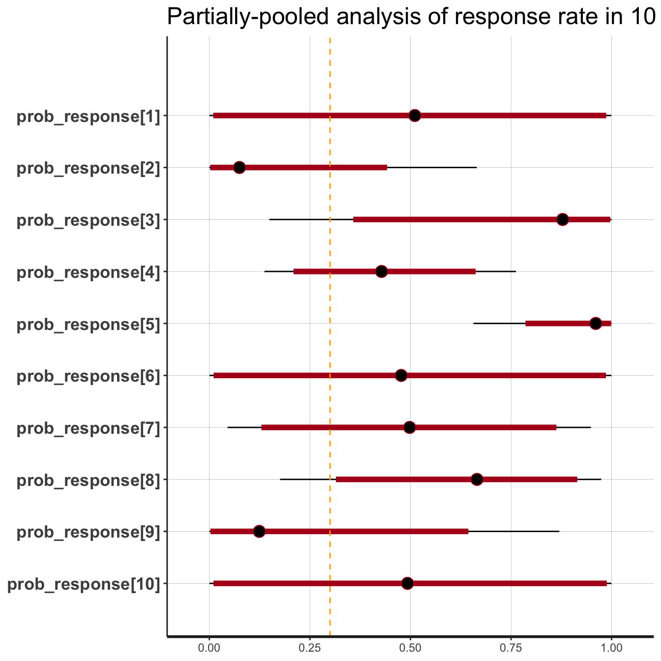
Prob(Response | D) in subgroup 3
We see that the inferred efficacy in subgroup 5 is very high. In contrast, efficacy is subject to more uncertainty in subgroup 4, but the majority of the mass clearly lies to the right of 30%.
trialr
trialr is available at https://github.com/brockk/trialr and https://CRAN.R-project.org/package=trialr
References
Thall, Peter F., J. Kyle Wathen, B. Nebiyou Bekele, Richard E. Champlin, Laurence H. Baker, and Robert S. Benjamin. 2003. “Hierarchical Bayesian Approaches to Phase II Trials in Diseases with Multiple Subtypes.” Statistics in Medicine 22 (5): 763–80. https://doi.org/10.1002/sim.1399.