Recap of the EffTox model
Thall & Cook (2004) introduced the EffTox design for dose-finding clinical trials where both efficacy and toxicity events guide dose selection decisions. This is in contrast to methods like 3+3 and CRM (O’Quigley, Pepe, and Fisher 1990), where dose selection is determined by toxicity events only. We provide a brief recap of EffTox here, but full details are given in (Thall and Cook 2004; Thall, Cook, and Estey 2006; Thall et al. 2014).
For doses \(\boldsymbol{y} = (y_1, ..., y_n)\), the authors define codified doses \((x_1, ..., x_n)\) using the transform
\(x_i = \log{y_i} - \sum_{j=1}^n \frac{\log{y_j}}{n}\)
The codified doses are used as the sole explanatory variables in logit models for the marginal probabilities of toxicity and efficacy:
\(\text{logit } \pi_T = \alpha + \beta x\)
\(\text{logit } \pi_E = \gamma + \zeta x + \eta x^2\)
Let \((Y_j, Z_j)\) be random variables each taking values \(\{0, 1\}\) respresenting the presence of efficacy and toxicity in patient \(j\).
Then the efficacy and toxicity events are associated by the joint probability function
\(Pr(Y = a, Z = b) = \pi_{a,b}(\pi_E, \pi_T) = (\pi_E)^a (1-\pi_E)^{1-a} (\pi_T)^b (1-\pi_T)^{1-b} + (-1)^{a+b} (\pi_E) (1-\pi_E) (\pi_T) (1-\pi_T) \frac{e^\psi-1}{e^\psi+1}\).
Normal priors are specified for the elements of the parameter vector \(\boldsymbol{\theta} = (\alpha, \beta, \gamma, \zeta, \eta, \psi)\).
At each dose update decision, the dose \(x\) is acceptable if
\(\text{Pr}\left\{ \pi_T(x, \boldsymbol{\theta}) < \overline{\pi}_T | \mathcal{D} \right\} > p_T\)
and
\(\text{Pr}\left\{ \pi_E(x, \boldsymbol{\theta}) > \underline{\pi}_E | \mathcal{D} \right\} > p_E\)
and is no more than than one position below the lowest dose-level given and no more than one position above the highest dose-level given. The net effect of these last two criteria is that untried doses may not be skipped in escalation or de-escalation. \(\underline{\pi}_E, p_E, \overline{\pi}_T, p_T\) are provided by the user as the trial scenario dictates.
The utility of dose \(x\), with efficacy \(\pi_E(x, \boldsymbol{\theta})\) and toxicity \(\pi_T(x, \boldsymbol{\theta})\) is
\(u(\pi_E, \pi_T) = 1 - \left( \left(\frac{1-\pi_E}{1-\pi_{1,E}^*}\right)^p + \left(\frac{\pi_T}{\pi_{2,T}^*}\right)^p \right) ^ \frac{1}{p}\)
where \(p\) is calculated to intersect the points \((\pi_{1,E}^*, 0)\), \((1, \pi_{2,T}^*)\) and \((\pi_{3,E}^*, \pi_{3,T}^*)\) in the efficacy-toxicity plain. I refer to these as hinge points but that is not common nomenclature.
At the dose selection decision, the dose-level from the acceptable set with maximal utility is selected to be given to the next patient or cohort. If there are no acceptable doses, the trial stops and no dose is recommended.
There are several published EffTox examples, including explanations and tips on parameter choices (Thall and Cook 2004; Thall, Cook, and Estey 2006; Thall et al. 2014).
The MD Anderson Cancer Center publishes software (Herrick et al. 2015) to perform calculations and simulations for EffTox trials. However, the software is available for Windows in compiled-form only. Thus, trialists cannot run the software on Mac or Linux unless using a virtual machine. Furthermore, trialists may not easily alter the behaviour of the model. Brock et al. (2017) describe a clinical trial scenario where some alteration of the default model behaviour would have been preferable. It was this that prompted the author to write the open-source implementation provided in trialr.
EffTox in trialr
We will work with the advanced prostate cancer example given in Thall et al. (2014). They investigate the five doses 1, 2, 4, 6.6 and 10 mcL/kg, seeking the best dose with
\(\text{Pr}\left\{ \pi_T(x, \boldsymbol{\theta}) < 0.3 | \mathcal{D} \right\} > 0.1\)
and
\(\text{Pr}\left\{ \pi_E(x, \boldsymbol{\theta}) > 0.5 | \mathcal{D} \right\} > 0.1\)
Thus, we have \(p_T = p_E = 0.1, \overline{\pi}_T = 0.3\) and \(\underline{\pi}_E = 0.5\).
The parameterisation for this trial is loaded by default in the MD Anderson EffTox app. This particular scenario is fit as a demonstration in trialr.
First, let us introduce our syntax for describing outcomes in phase I/II dose-finding trials, first described by Brock et al. (2017). We use integers to denote the dose-level given to a patient or cohort of patients; and strings of the letters E, T, N & B to represent the outcomes of patients treated at that dose that experienced efficacy, toxicity, neither or both, respectively. Clusters of these characters can be concatinated to reflect the outcomes of successive cohorts.
To study the method, let us imagine that we have treated six patients in two cohorts of three at dose-levels 1 and 2 respectively:
| Patient | Dose-level | Toxicity | Efficacy |
|---|---|---|---|
| 1 | 1 | 0 | 0 |
| 2 | 1 | 0 | 0 |
| 3 | 1 | 0 | 1 |
| 4 | 2 | 0 | 1 |
| 5 | 2 | 0 | 1 |
| 6 | 2 | 1 | 1 |
We fit Thall and Cook’s demonstration model to these outcomes, setting the random seed for reproducibility, using the call:
library(trialr)

outcomes <- '1NNE 2EEB'
fit <- stan_efftox_demo(outcomes, seed = 123)
fit## Patient Dose Toxicity Efficacy
## 1 1 1 0 0
## 2 2 1 0 0
## 3 3 1 0 1
## 4 4 2 0 1
## 5 5 2 0 1
## 6 6 2 1 1
##
## Dose N ProbEff ProbTox ProbAccEff ProbAccTox Utility Acceptable ProbOBD
## 1 1 3 0.402 0.088 0.333 0.927 -0.342 TRUE 0.0465
## 2 2 3 0.789 0.103 0.943 0.921 0.412 TRUE 0.2625
## 3 3 0 0.929 0.225 0.984 0.718 0.506 TRUE 0.2077
## 4 4 0 0.955 0.315 0.983 0.617 0.420 FALSE 0.0620
## 5 5 0 0.964 0.372 0.980 0.561 0.349 FALSE 0.4213
##
## The model recommends selecting dose-level 3.
## The dose most likely to be the OBD is 5.
## Model entropy: 1.36As with the CRM models, the default print method for EffTox models tabulates patient data and then dose-level data. We see that dose-level 3 is recommended for the next cohort, offering the projected best trade-off between efficacy and toxicity probabilities. We see that dose-levels 4 and 5 are unacceptable. This is because dose-level 3 has not yet been given. No doses are inferred to be too toxic or inefficacious yet.
More generally, the function stan_efftox can be used to fit EffTox models. The above call is simply short-hand for:
fit <- stan_efftox(outcomes,
                   real_doses = c(1.0, 2.0, 4.0, 6.6, 10.0),
                   efficacy_hurdle = 0.5, toxicity_hurdle = 0.3,
                   p_e = 0.1, p_t = 0.1,
                   eff0 = 0.5, tox1 = 0.65,
                   eff_star = 0.7, tox_star = 0.25,
                   alpha_mean = -7.9593, alpha_sd = 3.5487,
                   beta_mean = 1.5482, beta_sd = 3.5018,
                   gamma_mean = 0.7367, gamma_sd = 2.5423,
                   zeta_mean = 3.4181, zeta_sd = 2.4406,
                   eta_mean = 0, eta_sd = 0.2,
                   psi_mean = 0, psi_sd = 1,
                   seed = 123)
These are the parameters identified in Thall et al. (2014). Refer to the published paper for information on the normal priors.
The fit object contains
fit$recommended_dose
## [1] 3This confirms that dose-level 3 is acceptable dose with maximal utility.
We can produce contour plots.
efftox_contour_plot(fit)
title('EffTox utility contours')
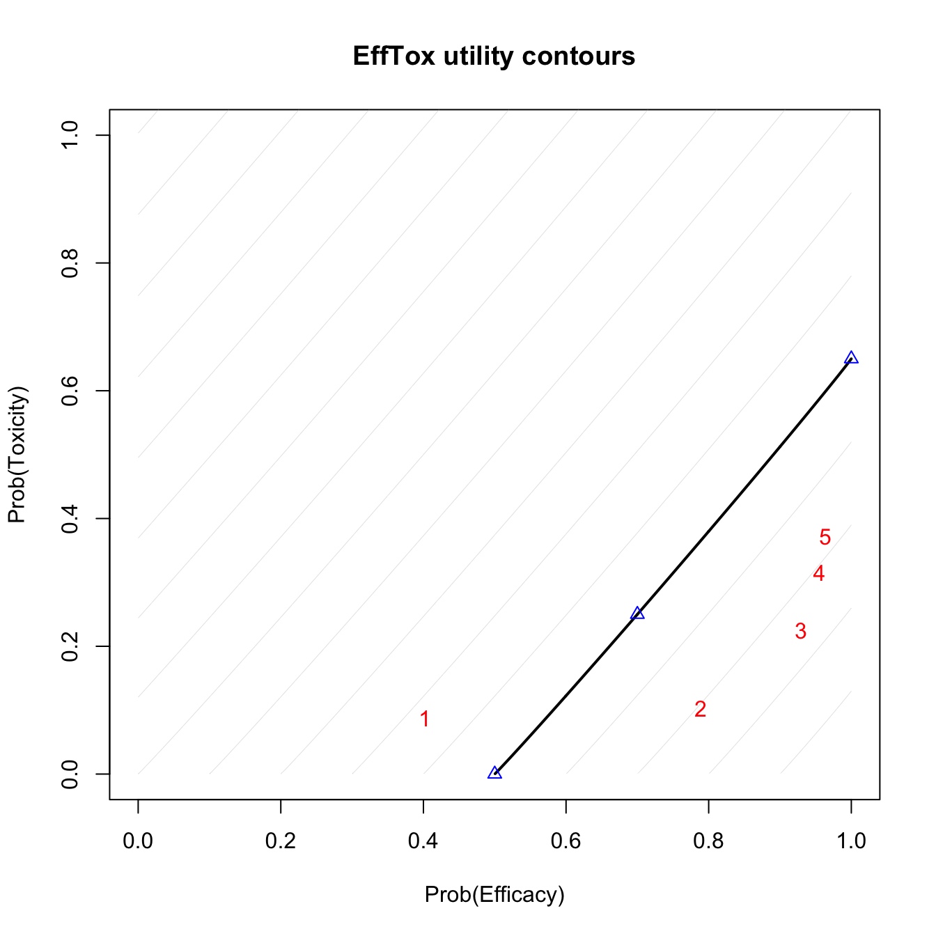
Utility contours after observing outcomes 1NEN 2NBE.
The blue points show the location of the hinge points on the neutral-uility (u=0) contour. The red numbers show the posterior means of the five dose-levels. Doses that are closer to the lower-right corner have higher utility. We see that dose-level 3 has the highest utility.
We can also produce posterior density plots of the dose utilities. For illustration, we will just plot the densities of the three acceptable doses. The package ggplot2 is required.
efftox_utility_density_plot(fit, doses = 1:3) +
  ggplot2::ggtitle("EffTox dose utility densities")
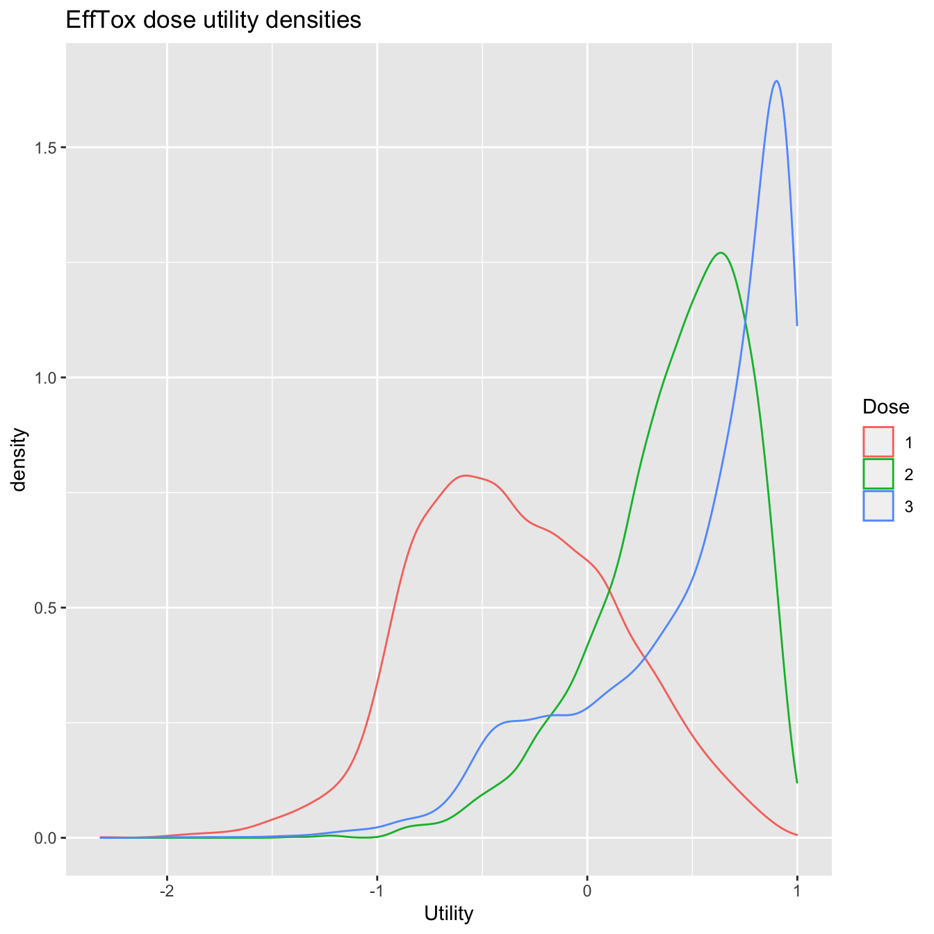
Utility densities after observing outcomes 1NEN 2NBE.
To further facilitate the analysis of dose utility, we provide means of calculating the dose superiority matrix.
knitr::kable(efftox_superiority(fit), digits = 2, row.names = TRUE)
| 1 | 2 | 3 | 4 | 5 | |
|---|---|---|---|---|---|
| 1 | NA | 0.95 | 0.88 | 0.82 | 0.78 |
| 2 | 0.05 | NA | 0.69 | 0.61 | 0.56 |
| 3 | 0.12 | 0.31 | NA | 0.50 | 0.47 |
| 4 | 0.18 | 0.39 | 0.50 | NA | 0.45 |
| 5 | 0.22 | 0.44 | 0.53 | 0.55 | NA |
The element in row \(i\) and column \(j\) shows \(\text{Prob(}u_j > u_i | \text{data)}\), where \(u_k\) is the utility of dose \(k\). We can be quite confident that dose 3 has higher utility than doses 1 and 2. In contrast, the model is much more vague about which is the superior of doses 3, 4 and 5. More data may be illuminating.
Simulation
We also provide a way to simulate EffTox trial scenarios. Simulation allows trialists to assess the performance of their design.
In addition to the parameters already described, the user must provide the true probabilities of efficacy and toxicity at each dose, and a vector of desired cohort sizes. For illustration, we simulate Scenario 1 under contour \(C_2\) in Table 1 of Thall et al. (2014). They use the EffTox parameterisation described above to investigate performance under true efficacy probabilities (0.2, 0.4, 0.6, 0.8, 0.9) and toxicity probabilities (0.05, 0.1, 0.15, 0.2, 0.4).
The preferable dose is calculated after the evaluation of each cohort and the following cohort is treated at the dose recommended. We provide the desired cohort sizes as a vector of integers via the cohort_sizes parameter. In the Thall example, they treat a maximum of 39 patients in thirteen cohorts of 3, thus we use cohort_sizes = rep(3, 13).
In the trialr EffTox implementation, the cohort sizes need not be constant. We can specify different cohort sizes, an option not possible in the official EffTox software. For instance, the investigators might want to re-evaluate the ideal dose after every patient in the early trial stages, where information is scarce. However, once a certain number of patient outcomes have been observed, they might prefer to revert to cohorts of three to avoid unnecessarily frequent analyses. To analyse the dose after each patient for the first 9 patients, followed by ten cohorts of three, we could use cohort_sizes = c(rep, 1, 9), rep(3, 10)).
Once again, we need a list of data to pass to the RStan sampler.
p <- efftox_solve_p(eff0 = 0.5, tox1 = 0.65, eff_star = 0.7, tox_star = 0.25)
dat <- list(
  num_doses = 5,
  real_doses = c(1, 2, 4, 6.6, 10),
  efficacy_hurdle = 0.5,
  toxicity_hurdle = 0.3,
  p_e = 0.1,
  p_t = 0.1,
  p = p,
  eff0 = 0.5,
  tox1 = 0.65,
  eff_star = 0.7,
  tox_star = 0.25,

  alpha_mean = -7.9593, alpha_sd = 3.5487,
  beta_mean = 1.5482, beta_sd = 3.5018,
  gamma_mean = 0.7367, gamma_sd = 2.5423,
  zeta_mean = 3.4181, zeta_sd = 2.4406,
  eta_mean = 0, eta_sd = 0.2,
  psi_mean = 0, psi_sd = 1,

  doses = c(),
  tox   = c(),
  eff   = c(),
  num_patients = 0
)
The elements in dat reflect the point from which each simulated trial iteration will commence. Note that num_patients, doses, tox and eff convey that no patients have yet been observed. This is not a constraint. Unlike the official EffTox software, users may simulate the commencement of a partially-observed EffTox trial by tailoring these four items. To simulate trials starting from a blank canvas, these four elemnts should be set as shown above.
The following code will run a simulation.
set.seed(123)
sims = efftox_simulate(dat, num_sims = 100, first_dose = 1,
                       true_eff = c(0.20, 0.40, 0.60, 0.80, 0.90),
                       true_tox = c(0.05, 0.10, 0.15, 0.20, 0.40),
                       cohort_sizes = rep(3, 13))
The doses recommended at the end of each simulated trial are recorded in the recommended_dose slot of the sims object. For instance, infer from the simulated trials the probability that each dose will be recommended using
Similarly, you can calculate the probability of each dose being given to a random patient using
and the mean number of patients being treated at each dose-level in each simulation
Simulation speed
The call to efftox_simulate will take about 25 minutes to run 100 iterations. This is much slower than the official Windows EffTox app, which would typically take a number of seconds rather than minutes. The official app is written in C++ and uses a fast numerical method for resolving Bayesian integrals with Gaussian priors called spherical radial integration, presented by Monahan & Genz (1997). In contrast, trialr delegates posterior sampling to rstan. The time it takes to run simulated EffTox trials in trialr is largely driven by the time it takes to run rstan::sampling many times. We are observing that MCMC is generally slower than spherical radial integration. However, it is also much more flexible. The trialr implementation of EffTox is easy to customise. Any aspect of the probability model may be changed by altering our open-source implementation. Non-normal priors may be used without any obligation to re-implement the prior-to-posterior analysis method. RStan handles the general model specification, rather than optimising for particular circumstances.
The process of simulating dose-finding trials is relatively computationally intensive because the dose update decision is made at the end of each cohort. In the above scenario, the dose decision is performed up to 13 times per iteration. When calling rstan::sampling, 4 chains of 2000 draws are used by default. Thus, 100 iterations of the above scenario involves \(100 \times 13 \times 4 = 5200\) chains sampled from the posterior distribution. Thus, if each call takes a fraction of a second (a sampled chain takes approximately 0.3s on my computer), the aggregate run-time is of the order of 20-30 minutes. Users can alter the number of chains used, the number of points per chain, and the amount of thinning by providing extra parameters via the ellipsis operator to efftox_simulate. These will then be forwarded to the rstan::sampling function.
Simulation is a costly exercise! Striking the balance between speed and flexibility is difficult. Sometimes a slow, flexibile method will be preferable to a fast, fixed method. It pays to hone parameters on small exploratory batches and commit to large jobs when ready.
trialr and the escalation package
escalation is an R package that provides a grammar for specifying dose-finding clinical trials. For instance, it is common for trialists to say something like ‘I want to use this published design… but I want it to stop once \(n\) patients have been treated at the recommended dose’ or ‘…but I want to prevent dose skipping’ or ‘…but I want to select dose using a more risk-averse metric than merely closest-to-target’.
trialr and escalation work together to achieve these goals. trialr provides model-fitting capabilities to escalation, including the EffTox method described here. escalation then provides additional classes to achieve all of the above custom behaviours, and more.
escalation also provides methods for running simulations and calculating dose-paths. Simulations are regularly used to appraise the operating characteristics of adaptive clinical trial designs. Dose-paths are a tool for analysing and visualising all possible future trial behaviours. Both are provided for a wide array of dose-finding designs, with or without custom behaviours like those identified above. There are many examples in the escalation vignettes at https://cran.r-project.org/package=escalation.
trialr
trialr is available at https://github.com/brockk/trialr and https://CRAN.R-project.org/package=trialr
References
Brock, Kristian, Lucinda Billingham, Mhairi Copland, Shamyla Siddique, Mirjana Sirovica, and Christina Yap. 2017. “Implementing the EffTox Dose-Finding Design in the Matchpoint Trial.” BMC Medical Research Methodology 17 (1): 112. https://doi.org/10.1186/s12874-017-0381-x.
Herrick, R, C Norris, JD Cook, and J Venier. 2015. “EffTox.” MD Anderson Cancer Center.
Monahan, John, and Alan Genz. 1997. “Spherical-Radial Integration Rules for Bayesian Computation.” Journal of the American Statistical Association 92 (438): 664–74.
O’Quigley, J, M Pepe, and L Fisher. 1990. “Continual Reassessment Method: A Practical Design for Phase 1 Clinical Trials in Cancer.” Biometrics 46 (1): 33–48. https://doi.org/10.2307/2531628.
Thall, PF, and JD Cook. 2004. “Dose-Finding Based on Efficacy-Toxicity Trade-Offs.” Biometrics 60 (3): 684–93.
Thall, PF, JD Cook, and EH Estey. 2006. “Adaptive Dose Selection Using Efficacy-Toxicity Trade-Offs: Illustrations and Practical Considerations.” Journal of Biopharmaceutical Statistics 16 (5): 623–38. https://doi.org/10.1080/10543400600860394.
Thall, PF, RC Herrick, HQ Nguyen, JJ Venier, and JC Norris. 2014. “Effective Sample Size for Computing Prior Hyperparameters in Bayesian Phase I-II Dose-Finding.” Clinical Trials 11 (6): 657–66. https://doi.org/10.1177/1740774514547397.