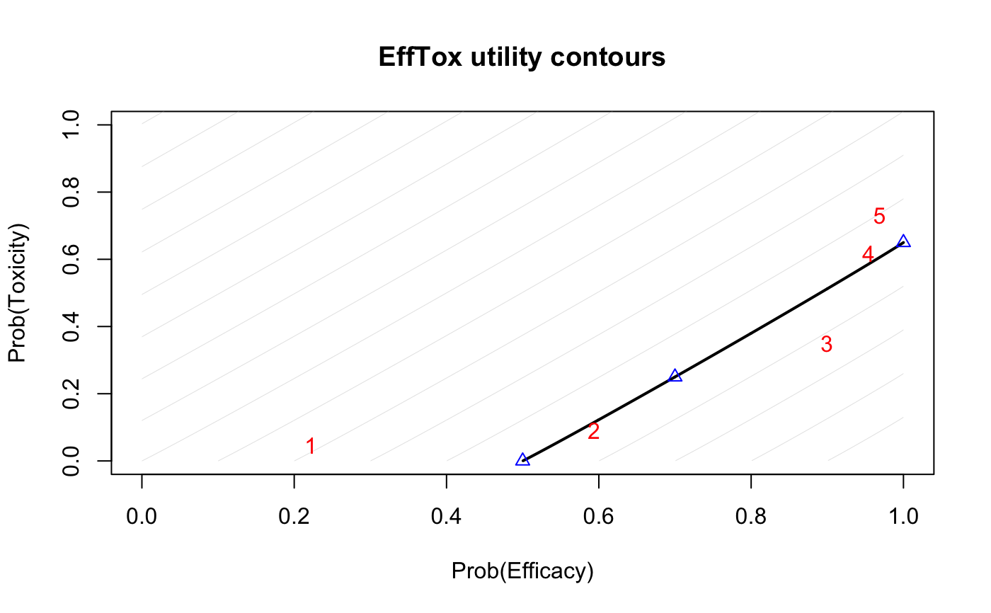
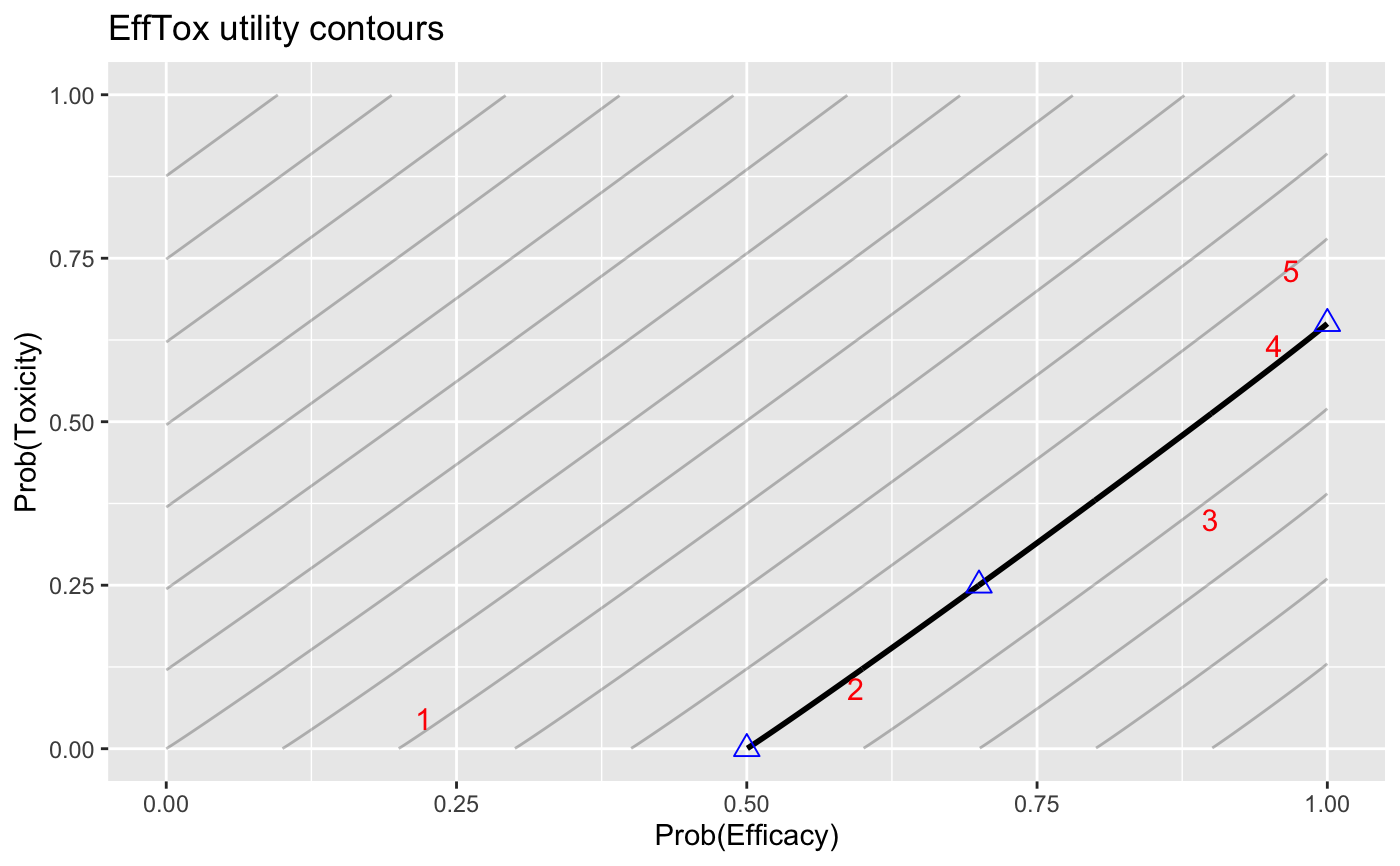
Plot EffTox utility contours. The probability of efficacy is on the x-axis and toxicity on the y-axis. The zero-utility curve is plotted bolder. The three "hinge points" are plotted as blue triangles. Optional Prob(Efficacy) vs Prob(Toxicity) points can be added; these are shown as red numerals, enumerated in the order provided.
efftox_contour_plot(
  fit,
  use_ggplot = FALSE,
  prob_eff = fit$prob_eff,
  prob_tox = fit$prob_tox,
  num_points = 1000,
  util_vals = seq(-3, 3, by = 0.2)
)
Arguments
| fit | An instance of |
|---|---|
| use_ggplot | logical, TRUE to use ggplot2. Defaults to FALSE to use standard R graphics. |
| prob_eff | vector of numbers between 0 and 1, containing the efficacy probabilities of extra points to add to the plot as points, e.g. the posterior mean efficacy probabilities of the doses under investigation. Paired with prob_tox, thus they should be the same length. Defaults to the values fitted by the model. Use NULL to supress. |
| prob_tox | vector of numbers between 0 and 1, containing the toxicity probabilities of extra points to add to the plot as points, e.g. the posterior mean toxicity probabilities of the doses under investigation. Paired with prob_eff, thus they should be the same length. Defaults to the values fitted by the model. Use NULL to supress. |
| num_points | integer for number of points to calculate on each curve. The default is 1000 and this should be plenty. |
| util_vals | A contour is plotted for each of these utility values.
The default is contours spaced by 0.2 between from -3 and 3,
i.e. |
Value
if use_ggplot = TRUE, an instance of ggplot; else no
object is returned. Omit assignment in either case to just view the plot.
See also
Examples
#> #> SAMPLING FOR MODEL 'EffTox' NOW (CHAIN 1). #> Chain 1: #> Chain 1: Gradient evaluation took 1.7e-05 seconds #> Chain 1: 1000 transitions using 10 leapfrog steps per transition would take 0.17 seconds. #> Chain 1: Adjust your expectations accordingly! #> Chain 1: #> Chain 1: #> Chain 1: Iteration: 1 / 2000 [ 0%] (Warmup) #> Chain 1: Iteration: 200 / 2000 [ 10%] (Warmup) #> Chain 1: Iteration: 400 / 2000 [ 20%] (Warmup) #> Chain 1: Iteration: 600 / 2000 [ 30%] (Warmup) #> Chain 1: Iteration: 800 / 2000 [ 40%] (Warmup) #> Chain 1: Iteration: 1000 / 2000 [ 50%] (Warmup) #> Chain 1: Iteration: 1001 / 2000 [ 50%] (Sampling) #> Chain 1: Iteration: 1200 / 2000 [ 60%] (Sampling) #> Chain 1: Iteration: 1400 / 2000 [ 70%] (Sampling) #> Chain 1: Iteration: 1600 / 2000 [ 80%] (Sampling) #> Chain 1: Iteration: 1800 / 2000 [ 90%] (Sampling) #> Chain 1: Iteration: 2000 / 2000 [100%] (Sampling) #> Chain 1: #> Chain 1: Elapsed Time: 0.097927 seconds (Warm-up) #> Chain 1: 0.061183 seconds (Sampling) #> Chain 1: 0.15911 seconds (Total) #> Chain 1: #> #> SAMPLING FOR MODEL 'EffTox' NOW (CHAIN 2). #> Chain 2: #> Chain 2: Gradient evaluation took 4.2e-05 seconds #> Chain 2: 1000 transitions using 10 leapfrog steps per transition would take 0.42 seconds. #> Chain 2: Adjust your expectations accordingly! #> Chain 2: #> Chain 2: #> Chain 2: Iteration: 1 / 2000 [ 0%] (Warmup) #> Chain 2: Iteration: 200 / 2000 [ 10%] (Warmup) #> Chain 2: Iteration: 400 / 2000 [ 20%] (Warmup) #> Chain 2: Iteration: 600 / 2000 [ 30%] (Warmup) #> Chain 2: Iteration: 800 / 2000 [ 40%] (Warmup) #> Chain 2: Iteration: 1000 / 2000 [ 50%] (Warmup) #> Chain 2: Iteration: 1001 / 2000 [ 50%] (Sampling) #> Chain 2: Iteration: 1200 / 2000 [ 60%] (Sampling) #> Chain 2: Iteration: 1400 / 2000 [ 70%] (Sampling) #> Chain 2: Iteration: 1600 / 2000 [ 80%] (Sampling) #> Chain 2: Iteration: 1800 / 2000 [ 90%] (Sampling) #> Chain 2: Iteration: 2000 / 2000 [100%] (Sampling) #> Chain 2: #> Chain 2: Elapsed Time: 0.091166 seconds (Warm-up) #> Chain 2: 0.059817 seconds (Sampling) #> Chain 2: 0.150983 seconds (Total) #> Chain 2: #> #> SAMPLING FOR MODEL 'EffTox' NOW (CHAIN 3). #> Chain 3: #> Chain 3: Gradient evaluation took 1.1e-05 seconds #> Chain 3: 1000 transitions using 10 leapfrog steps per transition would take 0.11 seconds. #> Chain 3: Adjust your expectations accordingly! #> Chain 3: #> Chain 3: #> Chain 3: Iteration: 1 / 2000 [ 0%] (Warmup) #> Chain 3: Iteration: 200 / 2000 [ 10%] (Warmup) #> Chain 3: Iteration: 400 / 2000 [ 20%] (Warmup) #> Chain 3: Iteration: 600 / 2000 [ 30%] (Warmup) #> Chain 3: Iteration: 800 / 2000 [ 40%] (Warmup) #> Chain 3: Iteration: 1000 / 2000 [ 50%] (Warmup) #> Chain 3: Iteration: 1001 / 2000 [ 50%] (Sampling) #> Chain 3: Iteration: 1200 / 2000 [ 60%] (Sampling) #> Chain 3: Iteration: 1400 / 2000 [ 70%] (Sampling) #> Chain 3: Iteration: 1600 / 2000 [ 80%] (Sampling) #> Chain 3: Iteration: 1800 / 2000 [ 90%] (Sampling) #> Chain 3: Iteration: 2000 / 2000 [100%] (Sampling) #> Chain 3: #> Chain 3: Elapsed Time: 0.077682 seconds (Warm-up) #> Chain 3: 0.058104 seconds (Sampling) #> Chain 3: 0.135786 seconds (Total) #> Chain 3: #> #> SAMPLING FOR MODEL 'EffTox' NOW (CHAIN 4). #> Chain 4: #> Chain 4: Gradient evaluation took 1.2e-05 seconds #> Chain 4: 1000 transitions using 10 leapfrog steps per transition would take 0.12 seconds. #> Chain 4: Adjust your expectations accordingly! #> Chain 4: #> Chain 4: #> Chain 4: Iteration: 1 / 2000 [ 0%] (Warmup) #> Chain 4: Iteration: 200 / 2000 [ 10%] (Warmup) #> Chain 4: Iteration: 400 / 2000 [ 20%] (Warmup) #> Chain 4: Iteration: 600 / 2000 [ 30%] (Warmup) #> Chain 4: Iteration: 800 / 2000 [ 40%] (Warmup) #> Chain 4: Iteration: 1000 / 2000 [ 50%] (Warmup) #> Chain 4: Iteration: 1001 / 2000 [ 50%] (Sampling) #> Chain 4: Iteration: 1200 / 2000 [ 60%] (Sampling) #> Chain 4: Iteration: 1400 / 2000 [ 70%] (Sampling) #> Chain 4: Iteration: 1600 / 2000 [ 80%] (Sampling) #> Chain 4: Iteration: 1800 / 2000 [ 90%] (Sampling) #> Chain 4: Iteration: 2000 / 2000 [100%] (Sampling) #> Chain 4: #> Chain 4: Elapsed Time: 0.086667 seconds (Warm-up) #> Chain 4: 0.073706 seconds (Sampling) #> Chain 4: 0.160373 seconds (Total) #> Chain 4:efftox_contour_plot(fit)title('EffTox utility contours')# The same with ggplot2 efftox_contour_plot(fit, use_ggplot = TRUE) + ggplot2::ggtitle('EffTox utility contours')#> Warning: Removed 23133 row(s) containing missing values (geom_path).#> Warning: Removed 500 row(s) containing missing values (geom_path).