The escalation package by Kristian Brock. Documentation
is hosted at https://brockk.github.io/escalation/
Introduction
Before reading this document on simulating dose-finding trials using
the escalation package, be sure to check out the README file. It explains
how to compose dose-finding designs using the flexible syntax provided
in escalation.
Once you have composed a design that appeals, you will want to learn about its operating performance by running many simulated trials, and possibly compare it to competing designs. That is the focus of this vignette. We study simulations because we believe they will predict the performance we can expect in reality. By operating performance, we mean:
- how often a design recommends a desirable dose;
- how many patients are treated;
- how many patients are treated at desirable doses;
- how many toxicities are seen;
- how often the design recommends stopping;
- how long trials take;
- and so on.
We are often interested both in the absolute levels of these
quantities, and how they compare to those of competing designs. When
comparing designs, we have an efficient method called
simulate_compare that examines the decisions of many design
on the same simulated patients to reduce Monte Carlo uncertainty.
Simulating trials in escalation
Simulations are run using the simulate_trials and
simulate_compare functions. These functions can be called
for any dose-escalation design in escalation. Specifying
dose-escalation models is the focus of the package README file.
simulate_trials runs simulations for a single particular
design. This is the focus of this vignette. In contrast,
simulate_compare compares several competing designs using
efficient methods that share notional patients across designs, ensuring
efficient comparisons. This topic is the focus of the Simulation Comparison
vignette.
The simplest example
Let us start with a very simple example by simulating performance of the 3+3 design in trial of five doses. We need to specify the unknown true probabilities of toxicity at the doses under investigation. Let us investigate:
true_prob_tox <- c(0.12, 0.27, 0.44, 0.53, 0.57)That is, doses 1 and 2 are what most clinicians would describe as tolerable, but doses 3, 4, and 5 are reasonably toxic. The 3+3 design does not target a particular probability of toxicity but empirically, the design tends to target doses with associated toxicity rates of 10-25%(Korn et al. 1994; Iasonos et al. 2008).
We must load the escalate package:
For the purposes of illustration, let us simulate a modest number of trials:
num_sims <- 20In reality, if we want to have confidence in the simulated results, we would tend to run thousands of iterations (Wheeler et al. 2019). We run a small number here so that this vignette compiles quickly.
We run simulations in our scenario using:
set.seed(123)

sims <- get_three_plus_three(num_doses = 5) %>%
  simulate_trials(num_sims = num_sims, true_prob_tox = true_prob_tox)
We set the random number generator seed in the example above so that results are (hopefully) reproducible. Despite setting the seed, the results could still vary across different operating systems or versions of R.
When printed to the screen, the sims object shows some
useful summary information:
sims
#> Number of iterations: 20
#>
#> Number of doses: 5
#>
#> True probability of toxicity:
#>    1    2    3    4    5
#> 0.12 0.27 0.44 0.53 0.57
#>
#> Probability of recommendation:
#> NoDose      1      2      3      4      5
#>   0.10   0.70   0.15   0.05   0.00   0.00
#>
#> Probability of administration:
#>      1      2      3      4      5
#> 0.3934 0.5082 0.0656 0.0328 0.0000
#>
#> Sample size:
#>    Min. 1st Qu.  Median    Mean 3rd Qu.    Max.
#>    3.00    8.25    9.00    9.15    9.75   18.00
#>
#> Total toxicities:
#>    Min. 1st Qu.  Median    Mean 3rd Qu.    Max.
#>    2.00    2.00    2.00    2.35    3.00    4.00
#>
#> Trial duration:
#>    Min. 1st Qu.  Median    Mean 3rd Qu.    Max.
#>   1.570   6.453   8.997   8.391  10.418  16.713
Each of those pieces of information is available progmatically by R functions. For instance, the probability of recommending each dose at the final analysis, inferred from these simulated iterations, is:
prob_recommend(sims)
#> NoDose      1      2      3      4      5
#>   0.10   0.70   0.15   0.05   0.00   0.00
Bear in mind that these probabilities are the result of a random process. If we run the simulations again with a different seed, we will get different results. Recall also that they are informed by a small number of simulated replicates so there will be considerable uncertainty around these statistics. If we ran a greater number of replicates, there would be less uncertainty.
We infer from the probabilities above that the design is likely to recommend one of the first two doses. However, there is a non-trivial probability that the design will recommend the third dose, which is probably too toxic, or recommend no dose at all.
How many patients are required?
summary(num_patients(sims))
#>    Min. 1st Qu.  Median    Mean 3rd Qu.    Max.
#>    3.00    8.25    9.00    9.15    9.75   18.00
We see that the simulated trials use between 3 and 24 patients, with an expected number of 9-12.
summary(n_at_recommended_dose(sims))
#>    Min. 1st Qu.  Median    Mean 3rd Qu.    Max.    NA's
#>     3.0     3.0     3.0     3.5     3.0     6.0       2
Of those, 3-4 at treated at the dose that is eventually recommended.
We can see how many patients are treated at each dose on a trial-by-trial basis. Here are the allocation counts for the first 10 trials:
n_at_dose(sims) %>% head(10)
#> # A tibble: 10 × 5
#>      `1`   `2`   `3`   `4`   `5`
#>    <int> <int> <int> <int> <int>
#>  1     3     6     0     0     0
#>  2     6     3     3     0     0
#>  3     3     6     0     0     0
#>  4     3     6     0     0     0
#>  5     6     6     0     0     0
#>  6     3     6     0     0     0
#>  7     6     6     3     0     0
#>  8     3     6     0     0     0
#>  9     3     3     0     0     0
#> 10     3     3     3     0     0
This information is aggregated in the probabilities of administation, i.e. the probability that an individual patient is treated at each dose-level:
prob_administer(sims)
#>          1          2          3          4          5
#> 0.39344262 0.50819672 0.06557377 0.03278689 0.00000000
We might be alarmed to learn that roughly 25% of patients are treated at doses 3-5, the doses we believe to be excessively toxic.
We can also see how many toxicities there were at each dose in the simulated trials (again, here are just the first 10):
tox_at_dose(sims) %>% head(10)
#> # A tibble: 10 × 5
#>      `1`   `2`   `3`   `4`   `5`
#>    <int> <int> <int> <int> <int>
#>  1     0     2     0     0     0
#>  2     1     0     2     0     0
#>  3     0     2     0     0     0
#>  4     0     2     0     0     0
#>  5     1     2     0     0     0
#>  6     0     3     0     0     0
#>  7     1     1     2     0     0
#>  8     0     2     0     0     0
#>  9     0     2     0     0     0
#> 10     0     0     2     0     0
and a summary of the total number of toxicities seen in the replicates:
We expect to see about 2-3 toxicities using this design in this scenario with no iteration producing more than 6 toxicities.
For convenience, simulations can be cast to a
tibble:
library(tibble)

as_tibble(sims) %>% head(12)
#> # A tibble: 12 × 12
#>    .iteration .depth  time dose     tox     n empiric_tox_rate mean_prob_tox
#>         <int>  <dbl> <dbl> <ord>  <dbl> <dbl>            <dbl>         <dbl>
#>  1          1      4  6.47 NoDose     0     0            0                 0
#>  2          1      4  6.47 1          0     3            0                NA
#>  3          1      4  6.47 2          2     6            0.333            NA
#>  4          1      4  6.47 3          0     0          NaN                NA
#>  5          1      4  6.47 4          0     0          NaN                NA
#>  6          1      4  6.47 5          0     0          NaN                NA
#>  7          2      5 12.6  NoDose     0     0            0                 0
#>  8          2      5 12.6  1          1     6            0.167            NA
#>  9          2      5 12.6  2          0     3            0                NA
#> 10          2      5 12.6  3          2     3            0.667            NA
#> 11          2      5 12.6  4          0     0          NaN                NA
#> 12          2      5 12.6  5          0     0          NaN                NA
#> # ℹ 4 more variables: median_prob_tox <dbl>, admissible <lgl>,
#> #   recommended <lgl>, true_prob_tox <dbl>
This returns a tidyverse tibble,
essentially a fancy data-frame, with the followign columns:
-
.iteration, the number of the simulated trial iteration, i.e..iteration == 1is the first simulated trial, etc; -
.depth, the cohort number. In the example above we see that the first trial ended after the second cohort but the second trial went as far as cohort 9; -
time, the time of the analysis, essentially the sum of all of the intra-patient recruitment times; -
dose, the numerical dose-level or ‘NoDose’ for the option to select no dose; -
tox, the number of toxicity events seen; -
n, the number of patients evaluated; -
empiric_tox_rate, simplytoxdivided byn; -
mean_prob_tox, if the method supports statistical estimation, the modelled mean toxicity probability; -
median_prob_tox, if the method supports statistical estimation, the modelled median toxicity probability; -
recommended, a logical to show whethet this dose (or stopping) was recommended by this iteration; -
true_prob_tox, the true yet unknown probability of toxicity in this simulated scenario.
Other selection models might add more columns to this object.
Getting the results in tibble format is liberating for
analysis and visualisation. For instance, using further
tidyverse packages, it is simple to visualise the
frequencies of the final model recommendations:
library(dplyr)
library(ggplot2)

as_tibble(sims) %>%
  filter(recommended) %>%
  ggplot(aes(x = dose, fill = dose)) +
  geom_bar()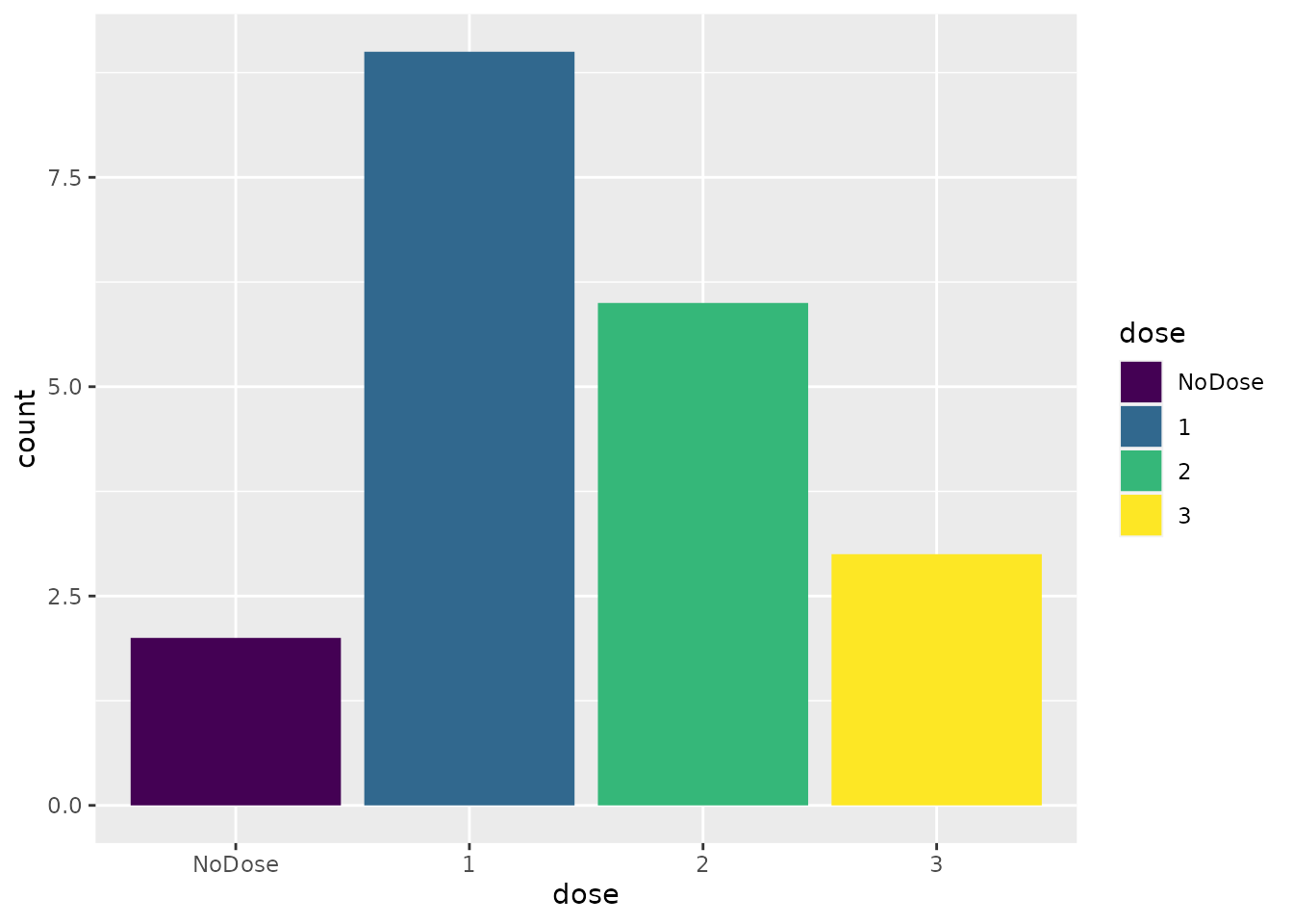
A more complex example
Let us consider now a model-based dose-finding approach in the same
scenario. We will investigate a CRM design, using the model from the
dfcrm package. Let us say that we are targeting a 25%
toxicity rate:
target <- 0.25and that our prior beliefs on the toxicity rates can be represented by:
skeleton <- c(0.05, 0.1, 0.25, 0.4, 0.6)i.e. we believe the third dose is the dose we seek.
The CRM design as provided by dfcrm offers no native
stopping behaviour. Let us say we are willing to use up to 12 patients.
How does performance of this simple design compare to the 3+3 above?
sims <- get_dfcrm(skeleton = skeleton, target = target) %>%
  stop_at_n(n = 12) %>%
  simulate_trials(num_sims = num_sims, true_prob_tox = true_prob_tox)

sims
#> Number of iterations: 20
#>
#> Number of doses: 5
#>
#> True probability of toxicity:
#>    1    2    3    4    5
#> 0.12 0.27 0.44 0.53 0.57
#>
#> Probability of recommendation:
#> NoDose      1      2      3      4      5
#>   0.00   0.20   0.35   0.40   0.05   0.00
#>
#> Probability of administration:
#>     1     2     3     4     5
#> 0.375 0.225 0.125 0.225 0.050
#>
#> Sample size:
#>    Min. 1st Qu.  Median    Mean 3rd Qu.    Max.
#>      12      12      12      12      12      12
#>
#> Total toxicities:
#>    Min. 1st Qu.  Median    Mean 3rd Qu.    Max.
#>    1.00    3.00    4.00    3.65    4.25    6.00
#>
#> Trial duration:
#>    Min. 1st Qu.  Median    Mean 3rd Qu.    Max.
#>   7.204  10.197  12.149  11.756  13.025  17.429
The first thing we note is that the CRM design is much less likely to
select dose 1 and more likely to select dose 2. If we believe that
efficacy is associated with toxicity (and we should if we are using the
CRM approach), then this is a good thing. Note, however, that comparing
separate simulations is not the most efficient method to compare
competing designs. A preferable method is to use
simulate_compare, demonstrated below.
However, our design has no method to stop if all doses are too toxic. We saw above that the 3+3 design occasionally recommended no dose. Thus, when comparing this CRM design to the 3+3, we are not comparing like with like. It is simple to add a stopping behaviour for excess toxicity:
sims <- get_dfcrm(skeleton = skeleton, target = target) %>%
  stop_at_n(n = 12) %>%
  stop_when_too_toxic(dose = 1, tox_threshold = 0.35, confidence = 0.8) %>%
  simulate_trials(num_sims = num_sims, true_prob_tox = true_prob_tox)

sims
#> Number of iterations: 20
#>
#> Number of doses: 5
#>
#> True probability of toxicity:
#>    1    2    3    4    5
#> 0.12 0.27 0.44 0.53 0.57
#>
#> Probability of recommendation:
#> NoDose      1      2      3      4      5
#>   0.00   0.25   0.45   0.20   0.10   0.00
#>
#> Probability of administration:
#>      1      2      3      4      5
#> 0.5250 0.1875 0.0875 0.1875 0.0125
#>
#> Sample size:
#>    Min. 1st Qu.  Median    Mean 3rd Qu.    Max.
#>      12      12      12      12      12      12
#>
#> Total toxicities:
#>    Min. 1st Qu.  Median    Mean 3rd Qu.    Max.
#>     2.0     3.0     3.0     3.2     4.0     5.0
#>
#> Trial duration:
#>    Min. 1st Qu.  Median    Mean 3rd Qu.    Max.
#>   5.347   9.121  10.778  10.824  12.453  16.080
We now see some trial iterations that stop and recommend no dose for further study. We cannot see from this scenario whether this design stops frequently enough because an appropriate decision in this scenario is to select one of the lowest two doses. We will research a scenario where all doses are too toxic below.
Given the fixed sample size, how many are treated at the dose that is eventually recommended
summary(n_at_recommended_dose(sims))
#>    Min. 1st Qu.  Median    Mean 3rd Qu.    Max.
#>     0.0     3.0     3.0     4.8     6.0    12.0
Similar to the 3+3 design, this CRM design treats 3-4 at the recommended dose. We might want to ensure that there are at least 6 patients at the recommended dose. How would that affect the operating characteristics?
sims <- get_dfcrm(skeleton = skeleton, target = target) %>%
  stop_at_n(n = 12) %>%
  stop_when_too_toxic(dose = 1, tox_threshold = 0.35, confidence = 0.8) %>%
  demand_n_at_dose(n = 6, dose = 'recommended') %>%
  simulate_trials(num_sims = num_sims, true_prob_tox = true_prob_tox)
As required, there are now at least 6 patients at the recommended dose:
summary(n_at_recommended_dose(sims))
#>    Min. 1st Qu.  Median    Mean 3rd Qu.    Max.    NA's
#>   6.000   6.000   6.000   6.789   6.000  12.000       1
So how does this affect the expected overall sample size?
sims
#> Number of iterations: 20
#>
#> Number of doses: 5
#>
#> True probability of toxicity:
#>    1    2    3    4    5
#> 0.12 0.27 0.44 0.53 0.57
#>
#> Probability of recommendation:
#> NoDose      1      2      3      4      5
#>   0.05   0.30   0.45   0.20   0.00   0.00
#>
#> Probability of administration:
#>      1      2      3      4      5
#> 0.4490 0.2857 0.1327 0.1224 0.0102
#>
#> Sample size:
#>    Min. 1st Qu.  Median    Mean 3rd Qu.    Max.
#>     3.0    12.0    15.0    14.7    18.0    21.0
#>
#> Total toxicities:
#>    Min. 1st Qu.  Median    Mean 3rd Qu.    Max.
#>    2.00    3.00    3.50    4.15    5.00    9.00
#>
#> Trial duration:
#>    Min. 1st Qu.  Median    Mean 3rd Qu.    Max.
#>   5.534  13.641  16.064  16.436  19.347  28.336
Pleasingly, the expected sample size only increases by about 3 patients. Obviously, the maximum increases by 6 patients.
Further refinements
The following behaviours apply to both simulate_trials
and simulate_compare.
Cohort size
All of the above simulations assume that patients are evaluated in cohorts of three. That assumption is made mainly by convention but naturally it is possible to change that.
We can adjust in simulations the way that simulated patients arrive
by providing a custom function via the
sample_patient_arrivals parameter. For instance, if we want
the model to recommend a new dose after every other patient, we can
specify that the sample_patient_arrivals function samples
patients in cohorts of two:
patient_arrivals_func <- function(current_data) cohorts_of_n(n = 2)

model <- get_dfcrm(skeleton = skeleton, target = target) %>%
  stop_at_n(n = 12) %>%
  stop_when_too_toxic(dose = 1, tox_threshold = 0.35, confidence = 0.8) %>%
  demand_n_at_dose(n = 6, dose = 'recommended')

sims <- model %>%
  simulate_trials(num_sims = num_sims, true_prob_tox = true_prob_tox,
                  sample_patient_arrivals = patient_arrivals_func)
The sample_patient_arrivals function samples the arrival
times of new patients for the next interim analysis. The new patients
will be added to the existing patients and the model will be fit to the
set of all patients. The function that simulates patient arrivals should
take as a single parameter a data-frame with one row for each existing
patient and columns including cohort, patient,
dose, tox, time (and possibly
also eff and weight, if a phase I/II or
time-to-event method is used). The provision of data on the existing
patients to sample_patient_arrivals allows the patient
sampling function to be adaptive. The function should return a
data-frame with a row for each new patient and a column for
time_delta, the time between the arrival of this patient
and the previous, like the cohorts_of_n function does:
cohorts_of_n(n = 5)
#>   time_delta
#> 1 0.99586980
#> 2 0.02669685
#> 3 0.67005583
#> 4 2.52444885
#> 5 1.88378957
Sampling the conclusion of partly-observed trials
The examples demonstrated so far simulate whole trials, from the
recruitment and evaluation of the first patient to the last. However,
simulate_trials will gladly simulate the culmination of
trials that are partly completed. We just have to specify the outcomes
already observed via the previous_outcomes parameter. Each
simulated trial will commence from those outcomes seen thus far.
For example, let us say that we have observed the first cohort of three already at dose 1, yielding one toxicities and two non-toxicities.
set.seed(123)

sims <- model %>%
  simulate_trials(num_sims = num_sims, true_prob_tox = true_prob_tox,
                  previous_outcomes = '1NTN')
The appearance of an early toxicity at dose 1 appear to make it more likely that a low dose will be recommended, as we might expect:
prob_recommend(sims)
#> NoDose      1      2      3      4      5
#>    0.0    0.4    0.6    0.0    0.0    0.0
The previous_outcomes can be described by the outcome
string method demonstrated above. They can also be provided via a
data-frame, with the following columns:
previous_outcomes <- data.frame(
  patient = 1:3,
  cohort = c(1, 1, 1),
  tox = c(0, 1, 0),
  dose = c(1, 1, 1)
)

set.seed(123)
sims <- model %>%
  simulate_trials(num_sims = num_sims, true_prob_tox = true_prob_tox,
                  previous_outcomes = previous_outcomes)
We have just described the trial starting point in two different ways. The simulated iterations should produce exactly the same results:
prob_recommend(sims)
#> NoDose      1      2      3      4      5
#>    0.0    0.4    0.6    0.0    0.0    0.0
Next dose
Likewise, we can also set the dose to be given to the next patient or
cohort of patients by specifying the next_dose parameter.
For example, if we want to commence our simulations at dose 5, we would
run:
sims <- model %>%
  simulate_trials(num_sims = num_trials, true_prob_tox = true_prob_tox,
                  next_dose = 5)
If omitted, the next dose is calculated by invoking the model on the prevailing outcomes, a set that may well be empty. In this setting, most models would opt to start at dose 1 but this may vary by method.
All model fits
In simulations, the dose selection model is fit to the prevailing
data at each interim analysis. By default, only the final model fit for
each simulated trial is returned. This is done to conserve memory. With
a high number of simulated trials, storing many model fits per trial may
cause the executing machine to run out of memory. However, you can force
this function to retain all model fits by specifying
return_all_fits = TRUE.
For example:
sims <- get_three_plus_three(num_doses = 5) %>%
  simulate_trials(num_sims = num_sims, true_prob_tox = true_prob_tox,
                  return_all_fits = TRUE)
We can verify that there are now many analyses per trial:
sapply(sims$fits, length)
#>  [1] 3 3 4 3 4 6 4 4 7 3 5 6 5 6 3 5 6 4 4 5
The multiple fits within a single simulated trial are distinguishable
in tibble view via the .depth column:
as_tibble(sims) %>% head(12)
#> # A tibble: 12 × 12
#>    .iteration .depth  time dose     tox     n empiric_tox_rate mean_prob_tox
#>         <int>  <dbl> <dbl> <ord>  <dbl> <dbl>            <dbl>         <dbl>
#>  1          1      1  0    NoDose     0     0            0                 0
#>  2          1      1  0    1          0     0          NaN                NA
#>  3          1      1  0    2          0     0          NaN                NA
#>  4          1      1  0    3          0     0          NaN                NA
#>  5          1      1  0    4          0     0          NaN                NA
#>  6          1      1  0    5          0     0          NaN                NA
#>  7          1      2  2.48 NoDose     0     0            0                 0
#>  8          1      2  2.48 1          1     3            0.333            NA
#>  9          1      2  2.48 2          0     0          NaN                NA
#> 10          1      2  2.48 3          0     0          NaN                NA
#> 11          1      2  2.48 4          0     0          NaN                NA
#> 12          1      2  2.48 5          0     0          NaN                NA
#> # ℹ 4 more variables: median_prob_tox <dbl>, admissible <lgl>,
#> #   recommended <lgl>, true_prob_tox <dbl>
In contrast to the previous usage of as_tibble(sims), we
see that there are now model fits at multiple fits within each simulated
trial .iteration. The rows at .depth == 1
reflect the initial model fit before any new patients are recruited,
essentially the starting point of this simulated trial. The rows at
.depth == 2 show the model fit after the first cohort of
patients, and so on.
Big trials
Designs must eventually choose to stop the trial. However, some
selectors, like those derived from get_dfcrm, offer no
default stopping method. You may need to append stopping behaviour to
your selector via something like stop_at_n or
stop_when_n_at_dose, etc. To safeguard against simulating
runaway trials that never end, the simulate_trials function
will halt a simulated trial after 30 invocations of the dose-selection
decision. To breach this limit, specify
i_like_big_trials = TRUE in the function call. However,
when you forego the safety net, the onus is on you to write selectors
that will eventually stop the trial, so be careful!
sims <- get_dfcrm(skeleton = skeleton, target = target) %>%
  stop_at_n(n = 99) %>%
  simulate_trials(num_sims = 1, true_prob_tox = true_prob_tox,
                  i_like_big_trials = TRUE)
num_patients(sims)
#> [1] 99